Most Excel users know their way around a pivot table. A pivot table can quickly summarize basic statistical information (with sums or averages, for example) and display that data in a more meaningful format.
But before you can start pivoting your data, you may need to rearrange your data —in other words, you need to “unpivot” your data.
How to Unpivot Excel
What does unpivot look like in Excel? Consider a basic example: a set of students each take a test every month for their algebra class. You want to be able to more closely analyze the performance of each student. However, you can’t do so by having a separate column for each month, which is the way that this data is most commonly tracked. When you build a pivot table from that data, there will be nine different fields with test scores—one for each month of the school year—and the pivot table won’t be able to calculate an annual total.

To unpivot excel, we need to make the data look longer instead of wider by creating an aggregated “month” column, as shown in the image below. With all of the months in one column, another column is created for the corresponding test scores of each student for each month.

So, how do we get started? First, we need to convert our data into a pivot table. The fastest way to do this is simply by pressing [CTRL] + T.

After we have our table, under “Get and Transform Data” group found in the “Data” tab, we’re going to click “From Table/Range.”

This will prompt Excel to open the Power Query Editor. Once in the Power Query Editor, we’re going to right-click on the “Name” column and select “Unpivot Other Columns.”

Upon doing so, you’ll now notice that the data is in the format that we want—a separate column has been created for the months and for the test scores. Now, all we have to do is re-name these new columns by right-clicking on the top of the columns.

Once we’re done renaming the columns, we’ll simply click “Close and Load” in the top left corner of the screen. This will create another sheet for us to use as the basis of our Excel pivots. If we decide to update our data and add, for example, the summer months if the students decided to take summer courses, we would only have to update our data in the original tab and right click and “Refresh” our data after the unpivot in the new tab.

The Next Step: Pivots
Now, we’ve achieved our goal: unpivot Excel data so that it’s in an acceptable format to create a pivot table. We’re not going to get into the specific “how-tos” of creating a pivot table in this article, but the most important step you can take before creating a pivot table is understanding what question you want to ask of your data and why. Creating a pivot table does little good if it’s not answering a pertinent question to your business. For example, based upon our student data, we might want to understand the average student test score per month to see if the students had difficulty with particular subjects.
The unpivot and pivots functions are not limited to Excel, of course. Pivot SQL is a common function across many industries with SQL servers. The process of a pivot SQL looks a lot different than an Excel pivot since it relies on a querying language, but the end goal is the same.
The Move Away from Unpivot Excel and Pivot Functions
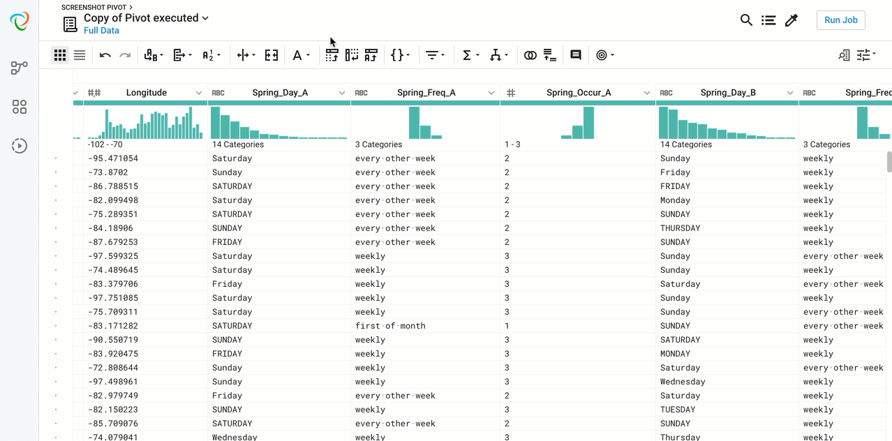
At Alteryx, there is love for a good pivot table. Excel unpivot and pivot are by all accounts the most powerful functions in Excel. But dealing in gigabytes worth of data with Excel can be unwieldy or even prohibitive. That’s why Designer Cloud has built a product that offers familiar pivot-table functionality, but with a superior visual interface and intelligent interactions. This means you get the multi-faceted view of the pivot table, without the unintuitive process. It also means you get the aggregation power of the unpivot Excel without the awkward practice of having to make multiple pivot tables.
As data lineage has become more important, we have seen a move away from unpivoting data in Excel, as the application makes it virtually impossible to track all of the transformations that have been made, when, and by whom. With Designer Cloud, every change is clearly listed at the right of your screen at all times.
An area where Designer Cloud sees the ubiquitous use of Excel dissipating most is in financial services and banking. The financial services industry historically has relied mostly on Excel as a basis for informing industry trends and critical calculations, like the Allowance for Loan and Lease Losses (ALLL). One of the most significant quarterly financial statement estimates, the ALLL, shows how much a bank has in reserve to offset bad debts, and it has an enormous impact on earnings and capital. ALLL is also a calculation that has been derived almost exclusively using Excel. In a December 2015 Mainstreet Technologies survey, over 64% of the financial institution respondents said they still use Excel, and 66% said they are seeking other tech solutions ahead of the FASB CECL release that rolls out in 2020.
Excel became institutionalized because it’s powerful and relatively easy. However, finance and other sectors are realizing that Excel has more than just dataset size limitations. It is estimated that almost 90% of spreadsheets have errors, made worse by the lack of controls as spreadsheets pass between coworkers. In fact, it was a relatively simple Excel cut and paste formula error in 2012 that caused JP Morgan to miscalculate a fund’s VaR risk profile to the tune of a $2B loss.
Above size limitations, nowhere is tracking and data lineage more important than in the financial services sector, where scrutinous audits and regulatory reporting rule. Designer Cloud makes tracking data simple, enabling real-time inventories of key data.
How Designer Cloud Transformed the Unpivot Excel Transform
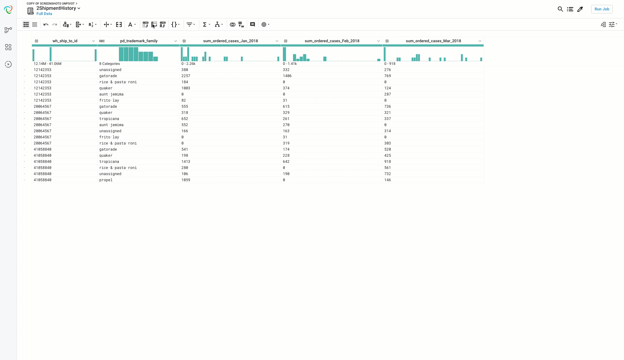
While Designer Cloud offers a predictive and visually pleasing way to execute a pivot transform, here we will focus on the Unpivot Excel command. The unpivot excel function is used most often when moving data from the data-entry stage to the analysis stage (e.g. normalizing data). Data entry is easiest when one assigns one row for each key (First Name) and one column for a data point (Hours Worked). This format makes for easy recording of data; however, aggregation and summation become far more difficult.
Designer Cloud reforms the data by merging one or more columns into key and value columns. Keys are the names of input columns, and value columns are the cell values from the source. Rows of data are duplicated, once for each input column. The unpivot Excel column can be applied to multiple columns in the same transform. All columns are un-pivoted into the same key and value columns. With data arranged this way, new aggregations can be made and new insights found. Designer Cloud’s solution for unpivot Excel function woes is truly for anyone who needs to organize their data efficiently and accurately.
Beyond the actual function of a pivot or unpivot Excel command, Designer Cloud has the built-in functionality to export directly to Tableau. Designer Cloud was built with Tableau users in mind: we know pivot/unpivot is an essential function, and we’ve made it easier and quicker to see your results, without employing the messiness of Excel. So if you are wondering how to unpivot data in excel, get started with Designer Cloud free trial!